pmcpy quickstart

# import necessary package
import pmcpy
import xarray as xr
import numpy as np
import pandas as pd
import matplotlib.pyplot as plt

load the raw output file from PartMC

# define the path to data
p = "../data/urban_plume_0001_00000002.nc"
pmc = pmcpy.load_pmc(p)

number concentration

print("overall number conc.:", pmc.get_num_conc(), "# m^{-3}")
print("diameter<=2.5um:", pmc.get_num_conc(pmc.get_aero_particle_diameter()<=2.5e-6), "# m^{-3}")
print("diameter>=2.5um:", pmc.get_num_conc(pmc.get_aero_particle_diameter()>=2.5e-6), "# m^{-3}")

overall number conc.: 8854807162.459946 # m^{-3}
diameter<=2.5um: 8854806282.274422 # m^{-3}
diameter>=2.5um: 880.1855249722205 # m^{-3}

aerosol mass concentration of selected species

# consider BC and OC only
aero_species_ls = ["BC","OC"]
print("BC and OC mass conc,:",
      pmc.get_aero_mass_conc(aero_species_ls),
      "kg m^{-3}")

# consider all species and dry species
all_aero_species = pmc.aero_species.copy()
dry_aero_species = all_aero_species.copy()
dry_aero_species.remove("H2O")

print("overall mass conc.:",
      pmc.get_aero_mass_conc(all_aero_species).sum(),
      "kg m^{-3}")
print("overall dry mass conc.:",
      pmc.get_aero_mass_conc(dry_aero_species).sum(),
      "kg m^{-3}")
print("PM2.5 mass conc. (with water):",
      pmc.get_aero_mass_conc(all_aero_species,
                             part_cond=(pmc.get_aero_particle_diameter()<=2.5e-6)).sum(),
      "kg m^{-3}")

BC and OC mass conc,: [6.53030409e-10 5.73984931e-09] kg m^{-3}
overall mass conc.: 2.2186891469474523e-08 kg m^{-3}
overall dry mass conc.: 1.316284475347949e-08 kg m^{-3}
PM2.5 mass conc. (with water): 2.2164289553077785e-08 kg m^{-3}

overall mass concentration

print("overall mass conc.:",
      pmc.get_mass_conc(dry=False), "kg m^{-3}")
print("overall dry mass conc.:",
      pmc.get_mass_conc(dry=True), "kg m^{-3}")
print("PM2.5 mass conc. (with water):",
      pmc.get_mass_conc(dry=False, part_cond=pmc.get_aero_particle_diameter()<=2.5e-6), "kg m^{-3}")

overall mass conc.: 2.2186891469474523e-08 kg m^{-3}
overall dry mass conc.: 1.316284475347949e-08 kg m^{-3}
PM2.5 mass conc. (with water): 2.2164289553077805e-08 kg m^{-3}

aerosol density

print("overall density.:",
      pmc.get_aero_density(dry=False), "kg m^{-3}")
print("overall dry density:",
      pmc.get_aero_density(dry=True), "kg m^{-3}")
print("PM2.5 density (with water):",
      pmc.get_aero_density(dry=False, part_cond=pmc.get_aero_particle_diameter()<=2.5e-6), "kg m^{-3}")

overall density.: 1179.020687087021 kg m^{-3}
overall dry density: 2265.3505453667535 kg m^{-3}
PM2.5 density (with water): 1178.3768174927013 kg m^{-3}

gas mixing ratio

gas_list = ['CO','O3']
pmc.get_gas_mixing_ratio(gas_list)

<xarray.DataArray 'gas_mixing_ratio' (gas_species: 2)>
array([354.311384,  43.069374])
Coordinates:
  * gas_species  (gas_species) int32 17 11
Attributes:
    unit:       ppb
    long_name:  mixing ratios of gas species

xarray.DataArray

'gas_mixing_ratio'

• gas_species: 2

• 354.3 43.07

  array([354.311384,  43.069374])

• Coordinates: (1)
  • gas_species
    (gas_species)
    int32
    17 11

    names :

    H2SO4,HNO3,HCl,NH3,NO,NO2,NO3,N2O5,HONO,HNO4,O3,O1D,O3P,OH,HO2,H2O2,CO,SO2,CH4,C2H6,CH3O2,ETHP,HCHO,CH3OH,ANOL,CH3OOH,ETHOOH,ALD2,HCOOH,RCOOH,C2O3,PAN,ARO1,ARO2,ALK1,OLE1,API1,API2,LIM1,LIM2,PAR,AONE,MGLY,ETH,OLET,OLEI,TOL,XYL,CRES,TO2,CRO,OPEN,ONIT,ROOH,RO2,ANO2,NAP,XO2,XPAR,ISOP,ISOPRD,ISOPP,ISOPN,ISOPO2,API,LIM,DMS,MSA,DMSO,DMSO2,CH3SO2H,CH3SCH2OO,CH3SO2,CH3SO3,CH3SO2OO,CH3SO2CH2OO,SULFHOX

    description :

    dummy dimension variable (no useful value) - read species names as comma-separated values from the 'names' attribute

    array([17, 11], dtype=int32)

• Attributes: (2)

  unit :

  ppb

  long_name :

  mixing ratios of gas species

mixing state index calculation

based on group_list

group_list = [['SO4','Cl','ARO1','ARO2','ALK1','OLE1',
                'API1','API2','LIM1','LIM2','Na'],
              ['BC','OC','OIN']]
pmc.get_mixing_state_index(group_list=group_list, diversity=False)

0.838104186813985

based on all species (without water)

pmc.get_mixing_state_index(drop_list=["H2O"], diversity=False)

0.6471920046172539

specific range of diameters and display diversity (\(D_\alpha\), \(D_\gamma\), \(\chi\))

pmc.get_mixing_state_index(drop_list=["H2O"],
                           part_cond=pmc.get_aero_particle_diameter()<=2.5e-6,
                           diversity=True)

(3.1876143541221267, 4.355134759609094, 0.6520198176412457)

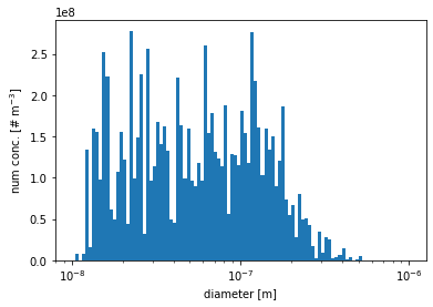
particle size distribution visualization (number concentration v.s. diameter)

overall number concentration

# get number distribution
aero_diameter = pmc.get_aero_particle_diameter()
num_conc_per_particle = pmc.ds["aero_num_conc"]

# setup the 111 bins ranged from 10^-8 to 10^-6
bins = np.logspace(-8,-6,2*50+1)

# plot the number distribution
plt.hist(aero_diameter, bins=bins, weights=num_conc_per_particle)
plt.xscale('log')
plt.xlabel('diameter [m]')
plt.ylabel(r'num conc. [# m$^{-3}$]')
plt.show()

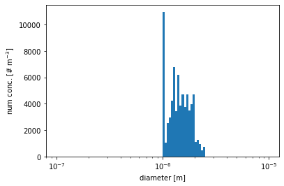
number concentration for particles with diameters between 1\(\mu\)m and 2.5\(\mu\)m

# get the diameters of all particles
aero_diameter = pmc.get_aero_particle_diameter()
# select particles with diameters between 1um and 2.5um
part_cond = (aero_diameter<=2.5e-6) & (aero_diameter>=1.0e-6)

aero_diameter_cond = aero_diameter[part_cond]
num_conc_per_particle_cond = pmc.ds["aero_num_conc"][part_cond]

# setup the 111 bins ranged from 10^-8 to 10^-6
bins = np.logspace(-7,-5,2*50+1)

# plot the number distribution
plt.hist(aero_diameter_cond, bins=bins, weights=num_conc_per_particle_cond)
plt.xscale('log')
plt.xlabel('diameter [m]')
plt.ylabel(r'num conc. [# m$^{-3}$]')
plt.show()

black carbon fraction in dry particles

# get dry species per parctile
all_aero_species = pmc.aero_species.copy()
dry_aero_species = all_aero_species.copy()
dry_aero_species.remove("H2O")
mass_per_dry_particle = pmc.ds["aero_particle_mass"]\
                           .sel(aero_species = pmc.aero_species_to_idx(dry_aero_species))\
                           .sum(dim="aero_species").values
# get black carbon mass per particle
bc_per_particle = pmc.ds["aero_particle_mass"]\
                     .sel(aero_species=pmc.aero_species_to_idx(["BC"])).values.reshape(-1)
bc_per_particle

array([0.00000000e+00, 0.00000000e+00, 0.00000000e+00, ...,
       5.78304546e-20, 0.00000000e+00, 0.00000000e+00])

bc_frac_per_dry_particle = bc_per_particle / mass_per_dry_particle
(bc_frac_per_dry_particle > 0.01).sum()

269

black carbon core volume

BC_density = pmc.ds["aero_density"].sel(aero_species = pmc.aero_species_to_idx(["BC"])).values
BC_density

array([1800.])

# volume = mass / density
pmc.ds["aero_particle_mass"].sel(aero_species = pmc.aero_species_to_idx(["BC"])).values / BC_density

array([[0.00000000e+00, 0.00000000e+00, 0.00000000e+00, ...,
        3.21280303e-23, 0.00000000e+00, 0.00000000e+00]])